Filtering Matrices
Filtering matrices are a construct that is useful for making LS estimates of a PSF from ground truth data. It is a Toeplitz matrix constructed from a parent array with the knowledge of the axes of the filtering kernel. Discrete correlation with the kernel can then be computed by matrix multiplication of the kernel with the filtering matrix. For vectors $x$ and $h$, the correlation $y = h \ast x$ can be written as
\[y = \begin{bmatrix} 0 & 0 & \cdots & 0 & x_0 & x_1 & \cdots & x_{k-1} & x_{k} \\ 0 & 0 & \cdots & x_0 & x_1 & x_2 & \cdots & x_{k} & x_{k+1} \\ \vdots & \vdots & & \vdots & \vdots & \vdots & & \vdots & \vdots \\ 0 & x_0 & \cdots & x_{n-k-1} & x_{n-k} & x_{n-k+1} & \cdots & x_{n-1} & x_n \\ x_0 & x_1 & \cdots & x_{n-k} & x_{n-k+1} & x_{n-k+2} & \cdots & x_n & 0 \\ \vdots & \vdots & & \vdots & \vdots & \vdots & & \vdots & \vdots \\ x_{n-k-1} & x_{n-k} & \cdots & x_{n-2} & x_{n-1} & x_{n} & \cdots & 0 & 0 \\ x_{n-k} & x_{n-k+1} & \cdots & x_{n-1} & x_n & 0 & \cdots & 0 & 0 \\ \end{bmatrix} \begin{bmatrix} h_{-k} \\ h_{-k+1} \\ \vdots \\ h_0 \\ \vdots \\ h_{k-1} \\ h_{+k} \end{bmatrix}\]
where the matrix is the filtering matrix of $h$ $F_h$ zero extended. The discrete convolution can be written analogously by reversing/reflecting $x$ or $h$. A filtering matrix for more than one dimensions can be used similarly with a flattened kernel.
TransferFunctions.FilteringMatrix — TypeFilteringMatrix{T,M,AA,KI,II} <: AbstractMatrix{T}A filtering matrix for the given M-dimensional array A and kernel indices kern. I.e. if K is an M-dimensional kernel with indices kern and F is the corresponding FilteringMatrix, then F * K[:] is the correlation of (or convolution if reflect(K)[:] where reflect(K) has the indices kern) of the K with A.
TransferFunctions.filtering_matrix — Functionfiltering_matrix(A, K, [border])Construct a FilteringMatrix of A with the kernel K such that the F'*K[:] produces a filtered vector of A.
If border is specified, the array is padded with the strategy border so that the full extent of the array A is kept in the filtering output.
julia> filtering_matrix(reshape(1:25, (5,5)), (-1:1, -1:1));

julia> filtering_matrix(reshape(1:25, (5,5)), OAs.OffsetArray(ones(3,3), -1:1, -1:1));

julia> filtering_matrix(reshape(1:9, (3,3)), (-1:1, -1:1), :symmetric)
9×9 filtering_matrix(border_array(reshape(::UnitRange{Int64}, 3, 3), :Symmetric), (3, 3)) with eltype Int64:
 5  4  5  2  1  2  5  4  5
 4  5  6  1  2  3  4  5  6
 5  6  5  2  3  2  5  6  5
 2  1  2  5  4  5  8  7  8
 1  2  3  4  5  6  7  8  9
 2  3  2  5  6  5  8  9  8
 5  4  5  8  7  8  5  4  5
 4  5  6  7  8  9  4  5  6
5 6 5 8 9 8 5 6 5K = OffsetArray(ones(11,11) ./ 121, -5:5, -5:5) # origin (0,0) must be contained in the kernel
F_A_inner = filtering_matrix(A, K)
A_corr_K_inner_flat = F_A_inner' * K[:]
A_corr_K_inner = reshape(A_corr_K_inner_flat, F_A_inner.interior)
@assert size(A_corr_K_inner) == (502, 502) # output of the correlation is reduced in size by the size of the kernelWe can extend the parent array by a border (see Border Arrays) to obtain the whole domain of A in the output of the correlation
F_A = filtering_matrix(A, K, :replicate)
A_corr_K_flat = F_A' * K[:]
A_corr_K = reshape(A_corr_K_flat, size(A))
@assert size(A_corr_K) == (512, 512) # whole domain of A is retained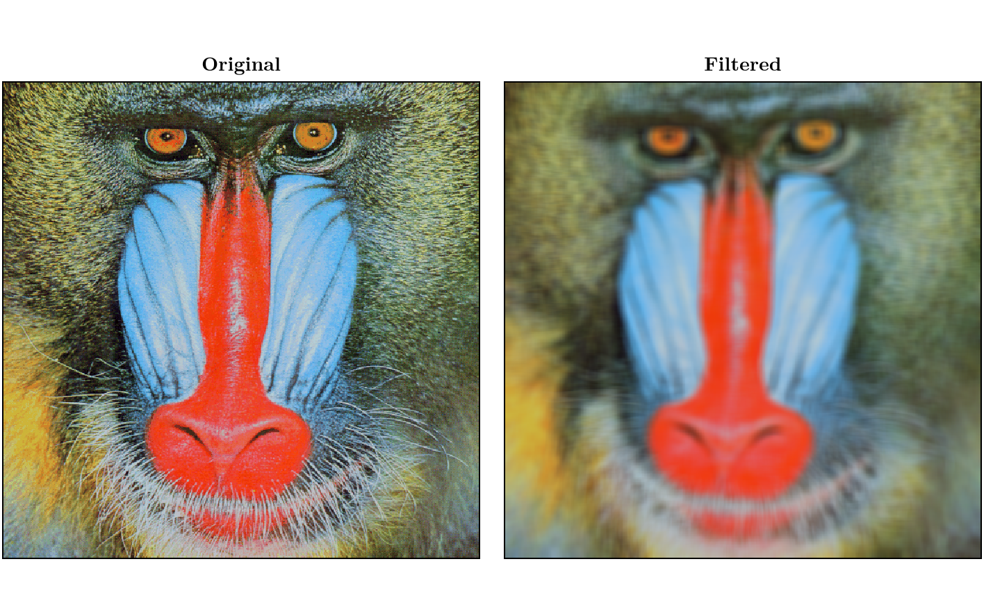
If we resize the image, we can see the structure of the filtering matrix for a matrix.
A_small = imresize(A, (20,20))
K_small = filtering_matrix(A_small, (-10:10, -10:10), :fill)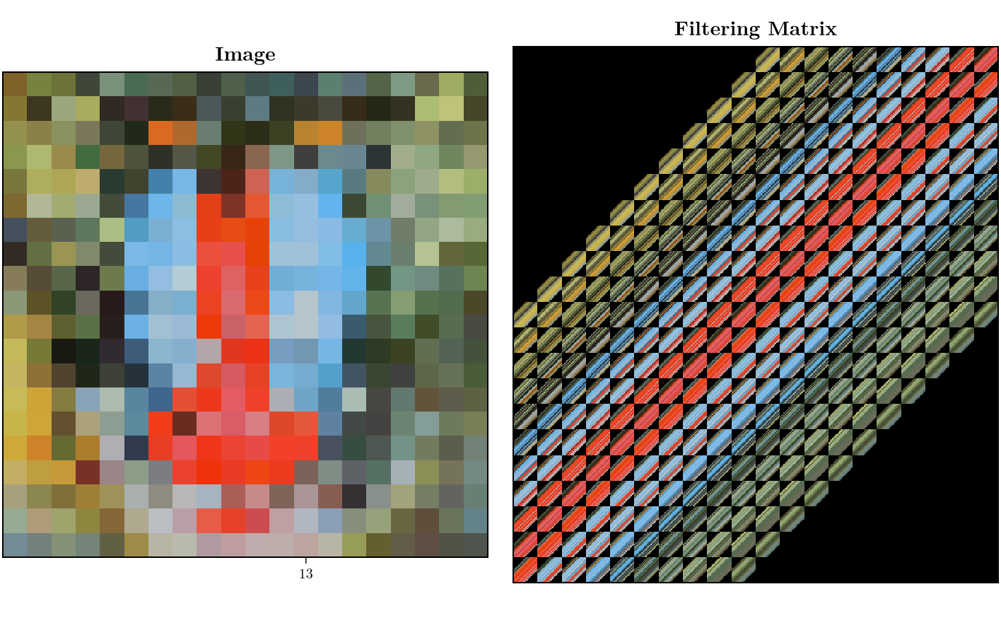
As can become apparent from the image, under some conditions on the border and the link between the length of A and K, the filtering matrix of a 2D matrix is a block circulant matrix.
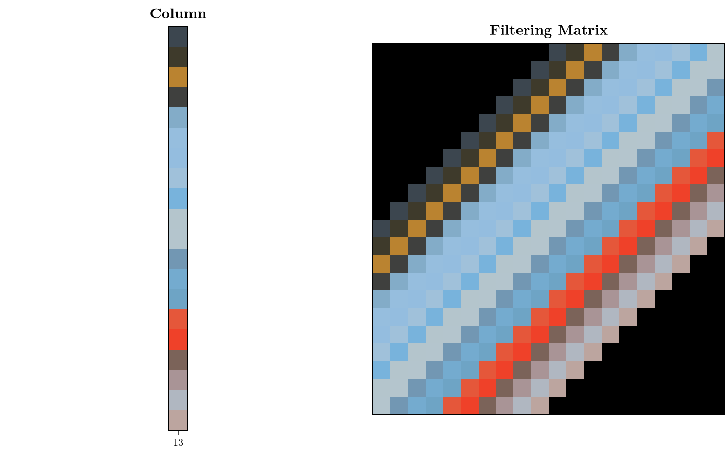
If we take a column slice from the image and create a filtering matrix from it, we can observe the structure of a filtering matrix of a vector.
A_col = A_small[:, 13]
K_A_col = filtering_matrix(A_col, (-10:10,), :fill)